For the Least Squares fit exercise, you have a three column file called “lsqdat.csv” that contains x, y and the error on y, sigma_y and you need to find the best fit straight line which goes through this data. Once you have that, you create a file called “teamname.csv” where “teamname” is the name of your team. For this exercise, given the equation of a straight line isy=mx+c there should be the gradient m on the first line, and the intercept c on the second line (one column, two rows).
All results should be submitted in .csv format, that is comma separated variable format so:-
1.0e0,23.4e0 2.0e0,24.7e0 2.6e0,32.43e0 ……..
or
1.35e2 2.43e2 ………
If everything is working well (and I am sure things will break down at some point during the day), then your results should be published on the big screen, so you can see how well you are doing relative to everybody else. The lower the value of Chi Squared that you produce the better.
For the second exercise, you are trying to predict the value of which will fit the supernova data. Because we are assuming that the Universe is flat (as confirmed by observations of the Cosmic Microwave Background) that means so that by giving your best bet for you have provided all the information we require. So we only need a single number.
The data for this is in the same google directory as for the straight line. The three columns are redshift (z), the difference between the absolute magnitude (m) and the apparent magnitude (M) which we call We don’t know the precise value of the absolute magnitude, or the precise value of the Hubble constant, so we have to treat this as a nuisance parameter, see notes, listen to presentation and ask the helpers or me for more guidance on this.
The third exercise is obtaining the redshift of galaxies from their photometric observations. The Sloan Digital Sky Survey obtains measurements of many millions of galaxies, but it cannot obtain detailed spectra, and hence redshifts, of all of them, or even the vast majority of them. Rather it measures their brightness in five different filter bands. I have provided you with a training set of 8000 galaxies with these five photometric (brightness) measurements, as well as their redshift, as well as a validation set for you to test your fitting algorithms on. Once you have an algorithm you are confident with, you can predict the redshifts of the galaxies in the test data set, and upload them via the form, this will be a one column list of 1000 redshifts (since there are 1000 sets of five brightnesses in the test file, but no redshifts.)
Please feel free to ask any questions you have, and ask me or the other helpers questions during the day.
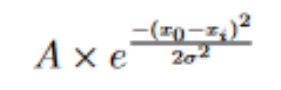
As these images were taken from Central London, there was a significant amount of light pollution that had to be accounted for in all the images. The effect of light pollution was found by fitting a gaussian distribution over a histogram of background pixel values, defined by:
The standard deviation of this fit accounts for this error on our data due to light pollution, where A is the amplitude, σ is the standard deviation, x0 is the centre of the distribution, and xi is the current data point we are generating a value for.
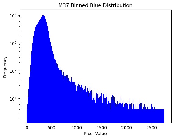
Looking at the histogram for the entire image for how many pixels of a certain brightness exist in the image, we can see that the grand majority of the data is quite dark, but not zero. We can assume that this is the light pollution, and the far more infrequent, brighter values are the stars.
In this histogram, the y-axis is logarithmic to show the low frequency data points. The pixel value is the brightnesss of a pixel, and the frequency is the number of pixels with that brightness found in the image.
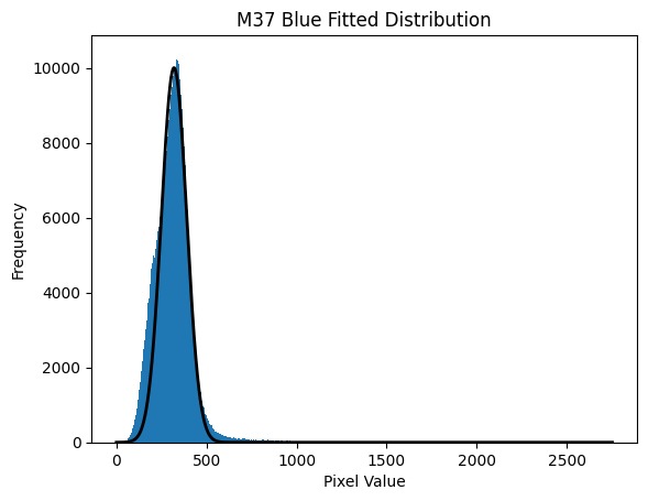
Applying an initial fit:
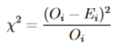
To test the goodness of our model data to our observed data, we implemented a chi-squared test, given by the below equation. A small chi squared value close to the range of pixel values we have implies a good fit.
Where O is observed data & E is expected data. We are using the Poisson Error squared as the denominator on our Chi Squared due to the Poisson nature of our observed values, a number of photons detected per exposure time.
To test how well our distribution fits, we employed a grid search method to vary each of the three parameters in our gaussian through an 11 x 11 x 11 grid, and calculating a chi-squared value for every combination of parameters in that grid. The smallest chi squared is then taken to be the centre, and a new grid is formed around it and the parameters are varied again. This is repeated until chi-squared stops decreasing, meaning we have found the minimum chi-squared value. The parameters of this best fit can be used to find the error due to light pollution.
def grid_search(unique_values, polluted_bins, ab, xob, wb):
    # Grid Jump Method

    # Define grid sizes

    dw = 10
    da = 100
    dxo = 20

    # Define data
    n = len(unique_values) #number of data points
    x = polluted_bins #our data
    y = generate_current_fit(polluted_bins) #fitted data

    # Initialize variables to store optimal parameters
    at = ab
    xot = xob
    wt = wb
    chisqmin = float('inf')

    # Perform grid search
    for l in range(-5, 6):
        w = max(0.0, wb + float(l) * dw)

        for k in range(-5, 6):
            a = max(0.0, ab + float(k) * da)

            for j in range(-5, 6):
                xo = max(0.0, xob + float(j) * dxo)

                # Compute chi-squared
                chisq = 0.0
                for i in range(n):
                    chisq += ((x[i] - a * np.exp(-((x[i] - xo) / 2*(w**2)) ** 2)) / max(1.0, x[i]))

                # Update optimal parameters if chi-squared is lower
                if chisq < chisqmin:
                    xot = xo
                    wt = w
                    at = a
                    chisqmin = chisq

                    print("New optimal parameters found:")
                    print("a =", a)
                    print("xo =", xo)
                    print("w =", w)
                    print("chi-squared =", chisq)

    print("Optimal parameters:")
    print("a =", at)
    print("xo =", xot)
    print("w =", wt)
    print("Minimum chi-squared =", chisqmin)

    return at, xot, wt

print("--------------BLUE--------------")
bat, bxot, bwt = grid_search(unique_values_blue, polluted_bins_blue, 13000, 455, 130)
print("-------------GREEN--------------")
gat, gxot, gwt = grid_search(unique_values_green, polluted_bins_green, 8000, 418, 150)
In the above code, w refers to the standard deviation σ.
Error Propagation
Written byNiharika Rath
Error analysis is obligatory to make valid scientific conclusions and to account for errors that gratuitously creep into the observations of any experiment. With our observations, we have 2 main sources of errors to account for, light pollution and a Poisson count error.
Following this, we proceeded to propagate the errors for the physical quantities used in plotting our HR diagram, namely the Flux, Magnitude and B-G values.
The √N is the error due to a Poisson counting error, where N is the count in a pixel. In our data, the count N is our flux F. The total error on the flux of all the pixels in the star is therefore √F. The error due to light pollution on the other hand is the width of the gaussian we fitted, σ. Adding these in quadrature gives:
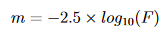
We calculated our magnitudes in each filter using the equation:
In order to propagate our errors through this, we used the error propagation equation of the form:
So our errors on magnitude have the form:
After subtracting the magnitudes in the green filter from the blue filter, the error on our B-G value is:
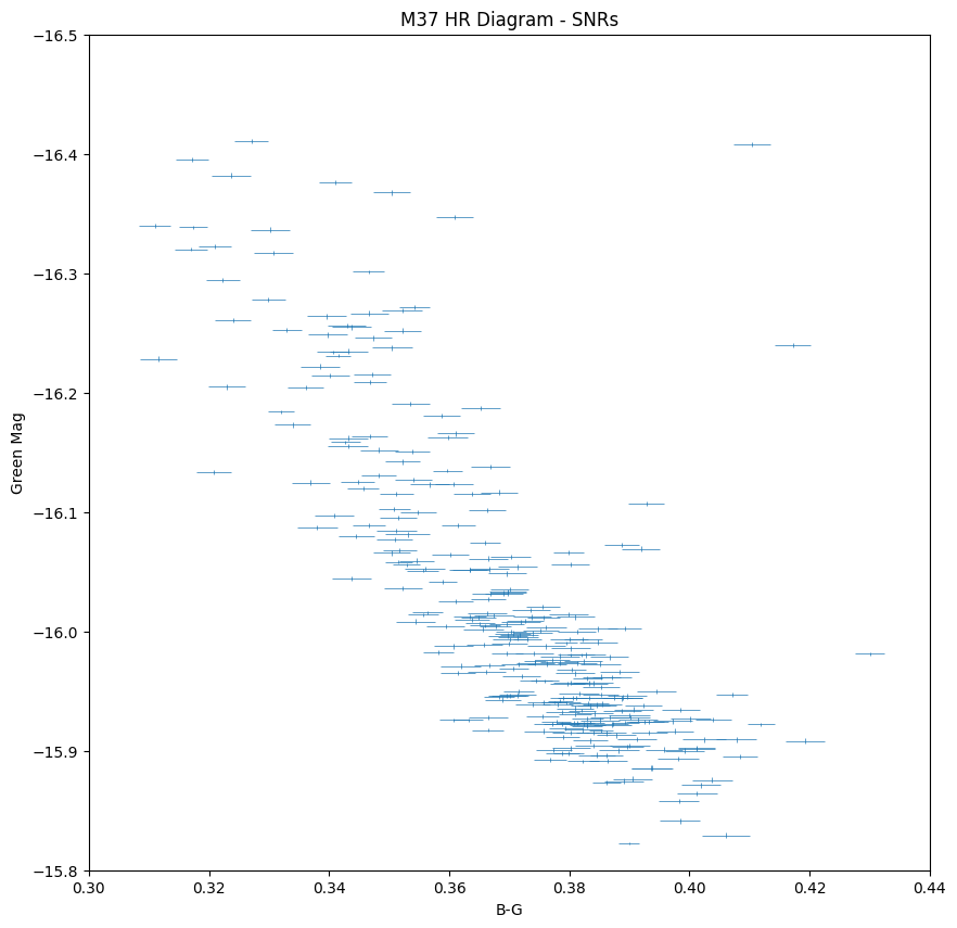
Using this, we attempt to prove the validity of our results and generate an HR diagram with values that match the literary ones, of course with an error associated with it:
Astronomers often use a quantity called the “signal to noise ratio” (S/N) to determine the accuracy of measurement or observation. This is the ratio of the signal (mean observation) divided by the noise (standard deviation of the observation). Oftentimes in similar projects we are working with Poisson statistics because we are only capturing some of the photons coming in from a distant source. For Poisson statistics, the standard deviation of a single measurement is the total number of counts.
For real astronomical observation, we must take into account that the star is observed on top of the sky background, which will produce an associated error in its measurement.
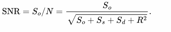
The S/N ratio of an observation for a CCD is given by
Where So is the shot-noise in the detected photo-electrons from the source, Ss is the shot-noise in the detected photo-electrons from the sky background, SD is the shot-noise in the thermally excited electrons, i.e the dark current, and R is the time-independent readout noise. Note, there is no square root on this term. The readout noise is the standard deviation in the number of electrons measured – it is not a Poissonian counting process.
In our project, however, the last two terms in the sum under the square root were ignored due to them having a negligible impact on the overall value. They are relatively small in the CCD documentation. Below is the line of code we used to calculate the ratio. It is taking a cutout of background and summing over all the pixels to get a total flux of the star. The rest of the propagation remains the same:
def calculate_snr(image, star_center, star_radius):
    # Define circular aperture for the star
    aperture_star = CircularAperture(star_center, r=star_radius)
    star_flux = aperture_star.to_mask(method="exact").cutout(image)

    # Define circular annulus for background
    aperture_bckgr = CircularAnnulus(star_center, r_in=star_radius+3, r_out=star_radius+10)
    bckgr_flux = aperture_bckgr.to_mask(method="exact").cutout(image)

    signal = np.sum(star_flux)

    # Calculate SNR
    snr = signal / np.sqrt( signal + np.sum(bckgr_flux) ) #/ len(bckgr_flux))

    return snr
Then adjusting “calculate flux errors” in our propagation code: