Unfortunately, London is plagued by a constant orange haze of light pollution. For the purposes of our project, light pollution harms our data as it adds a seemingly random value to all areas of the image, making it impossible to read the actual brightness of celestial bodies.
In order to remove the noise pollution, there are a few possible methods one could take. We tried two methods with varying degrees of success.
When taking the photos of each celestial body, we included an extra offset shot of the nearby sky. This shot was to provide us with a reference from which we could determine values to remove from our main photos, in order to remove the noise.
Method 1 – Minima removal
The simplest method of using the offset image is to compare each image with the offset image and generating an array of minima between the two images, as shown below.
Figure 1 – Code in order to generate a “mud” and remove it from the original image.
As described, the code generates an image showing the minima between the main images and the offset image, then subtracts this ‘mud’ from the original image to remove the noise pollution. The function backround_removal also needs error handling for underflow errors, as when values go below zero, they wrap back around to the maximum 32 bit integer. This can be avoided by implementing an if statement that checks if any values drop below zero, and returns them to zero.
However, as is now visible, artifacts in the form of dark holes appear on the image with the mud removed that line up with the stars visible in the offset image. In an ideal scenario, you would attempt to find a patch of sky with as few stars as possible in order to avoid this.
Figure 2 – The “Mud”. Note how the holes line up with the brightest stars in Figure 2 below.Figure 3 – The offset image, which lines up with the holes in the mud
Method 2 – Gradient Removal
n order to get rid of the artifacts, we instead found the gradient between the offset image and the 10 images, and from this we generated a noise map that represented the background in each image. Adding another error handler to avoid underflow errors, we then subtract the noise map from the original image, resulting in a clean, artifact free image from which we can extract data.
Figure 4 -The alternate method, generating a 2D background image that can then be subtracted from the original.Figure 5 – The noisemap generated by figure 3. As you can see, there are no visible stars left to cause artifacts, just a map of the skies brightness levels.Figure 6 – One of the final images with no background.
In this post, the concept of the hot pixels will be analyzed, the importance of removing the hot pixels from the FITS files will be emphasized and parts of the coding and the reasoning behind the steps followed will be explained.
What are the hot pixels and how are they obtained?
Hot pixels are single sharp pixels located at random locations of common images taken by digital cameras. They are points that do not react linearly to incident light captured by the lens. An important feature of the hot pixels is that they appear in the same location regardless the frame. This means they do not move, and they remain at a fixed position.
Hot pixels are caused due to electrical charges which appear into the sensor well of the camera’s lens. Since they are very sharp, and they are individual extremely bright pixels, they cannot be observed while looking at the image taken. However, they are very easy to determine while zooming at the images closely during processing, especially if the background of the image is very dark, such as the images taken from a telescope. They can also be visible when the sensor’s temperature increases or at very high ISOs[1]. The weather conditions during the photoshoot also have impact on the existence of the hot pixels since, if the temperature of the surroundings is high, it is ideal for their formation of hot pixels on the lens during the shoot. Finally, they tend to appear far more often in long exposure images. The reasoning behind the formation of the hot pixels is that while capturing less light from the scenery in the given moment, the patterns obtained by the camera sensor are comparatively stronger in that specific moment. Lenses and camera sensors get hotter and hotter as they use long exposures.
Why & how to remove hot pixels?
It is very important to remove the hot pixels from an image. The main reason is that it affects the image significantly during close viewing or printing. The only way they can be removed is by following a processing method after the image is taken. This can either happen through photo editing or coding. In this particular article, the second method will be analyzed and explained in detail.
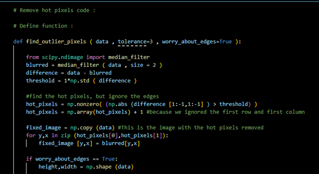
Figure 1- defining the function that will find the hot pixels of the FITS files. In this part of the code, median filter is being used, however, it can be replaced by a gaussian filter instead.
On Figure 1, the function that determines the hot pixels of each FITS file must be defined. In the first part of the code, the edges must be ignored, and they will be found separately later on. In order to understand the purpose behind it, we need to imagine the filter being a square with the center passing from every point of the image obtained. As the detector approaches the edges of the image, the corners of the square filter will exceed the limits and therefore the values they will obtain will be set by Python to zero, which affects the rest of the data (median/Gaussian filter).
Figure 2- Finding the hot pixels at the edges.
As indicated in the Figure 2 above, the next step of the code is to find the pixels on the edges of the image, but not the corners. Repeat the process for the left and right edges, top and bottom.
The next step is to find the hot pixels of the image at its four corners. The code used is very similar to the one used to determine those at the edges and can be indicated in the Figure 3 below:
Figure 3- Finding the hot pixels at the four corners of the image.
Using the previous Figures, the hot pixels can be obtained. Since the code would be required to be repeated for all images in order for them to get stacked, a part that repeats the following method can be introduced, which keeps the code simple and neat. However, the easiest method is to simply repeat the code for each FITS file of each cluster. A suggestion can be found below on Figure 4:
Figure 4 – Removing the hot pixels for or images before stacking.
When the data of the star clusters are collected using a CCD camera, the data is saved as a FITS file. To handle this FITS file in python, first, we need to understand what FITS files are. FITS (Flexible Image Transport System) is a file format designed to store, transmit, and manipulate the data saved on the file. The data stored in a fits file is multi-dimensional, like a 2D array. The pixel data from the camera is stored as a 2D or 3D array depending on the type of image. For example, if the data is monochrome, it is stored as a 2D array; if it is RGB, it is stored as a 3D array. The image metadata is stored as headers in ASCII format, which is readable by humans.
Handling FITS file in Python
To handle the FITS file in python, we first need to install a package called AstroPy. AstroPy is installed using the command line function on our compiler, which is python. We also install other valuable packages like photutils which detect stars and their positions on the image.
Figure 1: Installing AstroPy Package using command line function.
In the command line, we use the pip command to install the latest version of AstroPy and other useful packages. Once the needed packages are installed, we must import all necessary packages onto the jupyter notebook. For example, to open the fits file, we need a specific function of astropy to handle fits; the fits function is imported from astropy.io, as shown in the code below.
import numpy as np
import matplotlib.pyplot as plt
from astropy.io import fits
from matplotlib.colors import LogNorm as log
from astropy.stats import SigmaClip
from photutils.background import Background2D, MedianBackground
Once the packages are imported, we import the fits file onto our jupyter notebook and save it to a variable, as shown in the code below. Every fits file is saved into different variables.
To ensure the fits files are imported correctly, we must also ensure that the fits files are saved in the same directory as the jupyter notebook. After importing the fits file onto a variable, as shown in the code above, we now need to open them to manipulate the data, which is done using the fits.open() function, as shown in the code below.
Once the fits file is opened onto a variable, we now need to extract the data and store it onto another variable so that the data can be manipulated. The code to extract data is shown in the code below.
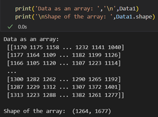
We extract the data as a 32-bit file (as shown in the code above) so that while manipulating the data, we avoid problems like stack overflow while processing the images. The extracted data can remove hot pixels, background, and stacking. This extracted data is a 2D array where every data point is the pixel value. We can also determine the shape of the array, which gives us an idea of the no. of pixels in the camera sensor.
Figure 2: Extracted data as an array and the shape of the array.
Figure 3: Raw data of M35B.
Figure 3 is the image representation of the extracted raw data of M35B in the log scale. This raw data contains hot pixels and a background, which is removed before stacking all the raw images collected.
Hello everyone! We are the Telescope Group 2023: Sof, Stel, Sara, Sarthak, Elvi, Matin, and Malcom. As part of our 3rd year research project, we are looking at different star clusters in London’s dark skies to measure the age of the stars within the clusters and produce a Hertzsprung-Russell (HR) diagram for them.
Here, we will be presenting how the FITS files, an astronomy file format, are handled in Python and the steps taken to get the HR diagram of the star clusters. The objects we have captured are the open clusters Messier 35, Messier 36, and Messier 37 on the night of 08/February/2023. We also observed the Orion Nebulae M42, and globular cluster M3.
The steps taken for our project each have a detailed blog post and are as follows:
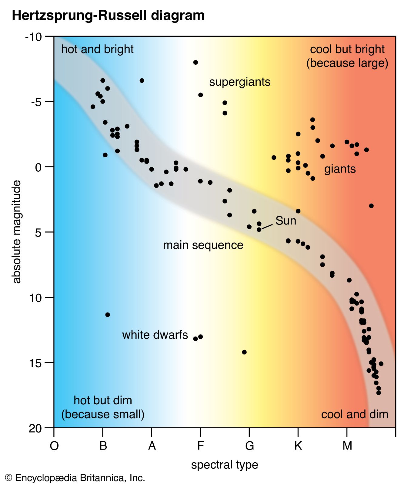
A Hertzsprung-Russell (HR) diagram is plot of stars showing the relationship between the stars’ absolute magnitude versus their effective temperatures. The absolute magnitude corresponds to the stars’ luminosities with negative values being brighter. The effective temperature can be shown using the stellar classification, where the stars from O to M correspond to decreasing temperate on the x-axis.1
An important feature in the HR diagram is the main sequence (MS), the region where the primary hydrogen-burning takes place within a star’s lifetime. Looking into detail where the MS ends, the “MS turn-off”, gives astronomers information about the age of the star cluster.
The general layout of the HR diagram can be seen below, where stars of greater luminosity are located at the top of the diagram, and stars with higher surface temperature are towards the left side of the diagram.
The data captured using the telescope at King’s gives us a FITS file, the most common digital file format in astronomy, and were captured with the blue and green filters attached. From that, we were able to open the files and get on with extracting the data. For this post, data from the M35 blue filter will be used. The raw image for M35_blue from Python can be seen:
Raw image of one of the data files for M35 Blue filter.
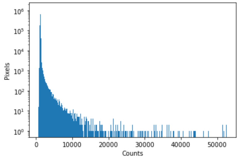
However, this raw image does not only contain the stars; it includes hot pixels captured by the filters and a background. The histogram below shows the numbers of counts vs the pixels of the image above:
Histogram of the data set above with the number of counts on the x-axis and the number pixels on the y-axis.
The brightest stars would be located on the histogram where the sharp peaks occur at the right of the curve. The highest peak of the histogram on the left side corresponds to the background of the image.
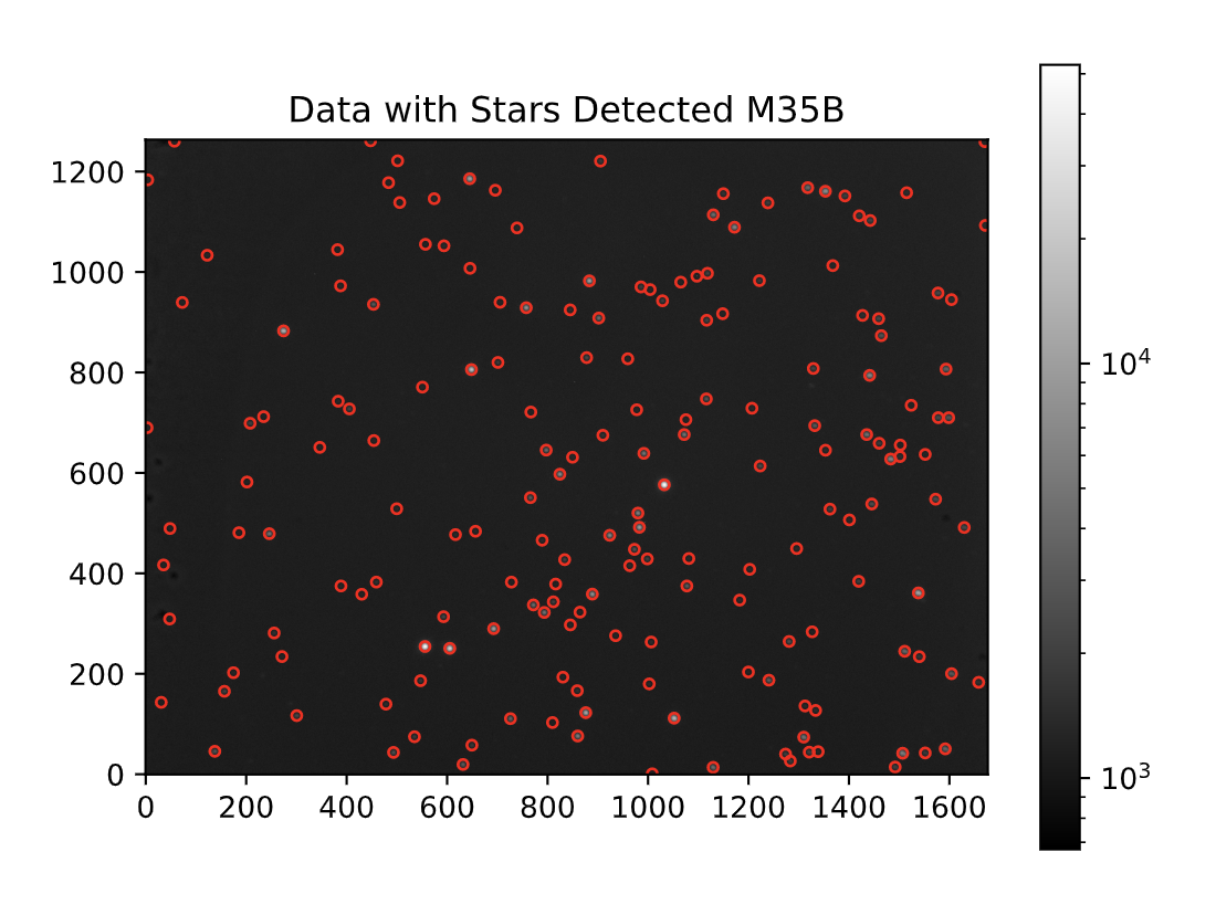
Next, the hot pixels needed to be removed from the image (detailed post here). Below is a picture showing the stars detected on the M35_Blue image after removing hot pixels using a code in Python:
Stars from M35_Blue are detected with a red circle around them.
The following procedure involved finding the background for it to be subtracted from each data set. The detailed methodology of background removal can be accessed here. The same steps were taken for each of the 10 data sets captured for M35_blue and M35_green. Now, the 10 images can be stacked to form:
Stacked image of M35 after removal of background and hot pixels in the blue filter.
The step afterwards was to identify the stars in the blue and green stacked images by comparing the two and see which stars overlap, i.e. correspond to the same star in the different filters.
After pairing the stars, the pixel counts of each star in both the blue and green images are found to compute the star’s apparent magnitudes (B and G). Finally, G vs. B-G is plotted, and this would form the observational HR-diagram of M35.
Observational HR diagram of open cluster M35.
The plot above displays HR diagram of M35, where the Main Sequence branch is clearly shown. The MS turn-off point is where the stars leave the MS and form “Giants” which are seen on the top right of the diagram. Since most stars are on the MS branch, and there are very few giants, this concludes that the open cluster M35 is fairly young.
Conclusion
This project aimed to produce an HR diagram of M35 starting from extracting the data in the FITS files to comparing the stars in the stacked images of the blue and green filter. The same methodology was applied to M36 and M37. This post provided a summary of the steps taken to reach the final result where details can be found in the appropriate separate posts.