Spectrum Response of the Atik 383L+ CCD through Astronomik Blue and Green Filters

Written by Niharika Rath

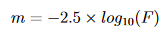
Plank’s law is used to calculate the energy per frequency of the light to get the number of photons per frequency.

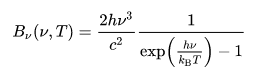
This is divided by the energy of a single photon to get the energy per frequency.This spectrum is then multiplied by the response curve of the camera (Quantum efficiency) and the response curve of the filter (RGB data from Astronomik). These curves represent the photon detection efficiency of the camera and filters at different frequencies.

We integrate over the response curve spectrum at each frequency to determine the total number of photons that get through the filter to reach the camera.The results are tabulated in a three column table giving the temperature of the light source and the number of photons that get through the blue and green filters to reach the camera sensor. This allows us to estimate the expected flux of the photons reaching the camera sensor and comparing it with our flux values to gauge the spectrum response through the filters. 

import numpy as np
from scipy.integrate import quad
import pandas as pd

# Planck's Law
def plancks_law(wavelength, temperature):
    h = 6.62607015e-34  # Planck's constant
    c = 3.0e8  # Speed of light
    k = 1.380649e-23  # Boltzmann constant

    wavelength_m = wavelength * 1e-9  # Convert wavelength from nm to meters
    frequency = c / wavelength_m
    energy = h * frequency

    exponent = h * c / (wavelength_m * k * temperature)
    intensity = (2 * h * c ** 2 / wavelength_m ** 5) / (np.exp(exponent) - 1)

    return intensity, energy

# Load transmission data for blue and green filters
blue_filter_data = np.loadtxt('Astronomik_Blue.csv', delimiter=',')
green_filter_data = np.loadtxt('Astronomik_Green.csv', delimiter=',')

# Load quantum efficiency data for camera
quantum_efficiency_data = np.loadtxt('QuantumEfficiency.csv', delimiter=',')

# Interpolate transmission and quantum efficiency data
def interpolate_data(wavelengths, data):
    return np.interp(wavelengths, data[:, 0], data[:, 1])

# Calculate total transmission through filters and camera response
def total_transmission(wavelengths):
    blue_transmission = interpolate_data(wavelengths, blue_filter_data)
    green_transmission = interpolate_data(wavelengths, green_filter_data)
    quantum_efficiency = interpolate_data(wavelengths, quantum_efficiency_data)
    return blue_transmission * quantum_efficiency, green_transmission * quantum_efficiency

# Function to compute the number of photons
def photons_per_frequency(wavelength, temperature, filter_type):
    intensity, energy = plancks_law(wavelength, temperature)
    total_trans_blue, total_trans_green = total_transmission(wavelength)
    if filter_type == 'blue':
        #filter_transmission = interpolate_data(wavelength, blue_filter_data)
        ppf =  intensity * total_trans_blue / energy
    elif filter_type == 'green':
        #filter_transmission = interpolate_data(wavelength, green_filter_data)
        ppf = intensity * total_trans_green / energy
    else:
        raise ValueError("Invalid filter type. Use 'blue' or 'green'.")
    return ppf

# Integrate the photons per frequency function
def integrate_photons(temperature, filter_type):
    return quad(photons_per_frequency, 300, 1000, args=(temperature, filter_type))[0]

# Generate table of temperatures and number of photons
temperatures = np.linspace(300, 2898, 50)
blue_photons = [np.log10(integrate_photons(temp, 'blue')) for temp in temperatures]
green_photons = [np.log10(integrate_photons(temp, 'green')) for temp in temperatures]

# Create a pandas DataFrame
results_df = pd.DataFrame({'Temperature (K)': temperatures,
                           'Blue Photons': blue_photons,
                           'Green Photons': green_photons})

print(results_df)

results_df.to_excel('photons_results.xlsx', index=False)
    Temperature (K)  Blue Photons  Green Photons
0        300.000000     -2.318112       1.661602
1        353.020408      3.861581       7.237948
2        406.040816      8.436797      11.367775
3        459.061224     11.962380      14.551051
4        512.081633     14.763506      17.080613
5        565.102041     17.043649      19.139870
6        618.122449     18.936303      20.849181
7        671.142857     20.533090      22.291338
8        724.163265     21.898716      23.524593
9        777.183673     23.080279      24.591446
10       830.204082     24.110034      25.523573
11       883.224490     25.020600      26.344953
12       936.244898     25.829487      27.074464
13       989.265306     26.552946      27.726677
14      1042.285714     27.203924      28.313305
15      1095.306122     27.792870      28.843782
16      1148.326531     28.328306      29.325821
17      1201.346939     28.817258      29.765833
18      1254.367347     29.265564      30.169010
19      1307.387755     29.678124      30.539835
20      1360.408163     30.059073      30.882066
21      1413.428571     30.411932      31.198891
22      1466.448980     30.739715      31.493040
23      1519.469388     31.045017      31.766922
24      1572.489796     31.330085      32.022465
25      1625.510204     31.596877      32.261500
26      1678.530612     31.847103      32.485577
27      1731.551020     32.082266      32.696061
28      1784.571429     32.303693      32.894152
29      1837.591837     32.512557      33.080915
30      1890.612245     32.711132      33.257261
31      1943.632653     32.897873      33.424104
32      1996.653061     33.074859      33.582161
33      2049.673469     33.242839      33.732109
34      2102.693878     33.402484      33.874557
35      2155.714286     33.554401      34.010054
36      2208.734694     33.699141      34.139098
37      2261.755102     33.837201      34.262215
38      2314.775510     33.969034      34.379655
39      2367.795918     34.095054      34.491880
40      2420.816327     34.215637      34.599227
41      2473.836735     34.331203      34.702005
42      2526.857143     34.441918      34.800501
43      2579.877551     34.548149      34.894978
44      2632.897959     34.650164      34.985676
45      2685.918367     34.748209      35.072818
46      2738.938776     34.842511      35.156581
47      2791.959184     34.933282      35.237210
48      2844.979592     35.020716      35.314822
49      2898.000000     35.104928      35.389646

Quantifying Light Pollution

Chi-Squared Test

Written by Matin Sharkawi

As these images were taken from Central London, there was a significant amount of light pollution that had to be accounted for in all the images. The effect of light pollution was found by fitting a gaussian distribution over a histogram of background pixel values, defined by:

The standard deviation of this fit accounts for this error on our data due to light pollution, where A is the amplitude, σ is the standard deviation, x0 is the centre of the distribution, and xi is the current data point we are generating a value for.

Looking at the histogram for the entire image for how many pixels of a certain brightness exist in the image, we can see that the grand majority of the data is quite dark, but not zero. We can assume that this is the light pollution, and the far more infrequent, brighter values are the stars.

In this histogram, the y-axis is logarithmic to show the low frequency data points. The pixel value is the brightnesss of a pixel, and the frequency is the number of pixels with that brightness found in the image.

Applying an initial fit:

To test the goodness of our model data to our observed data, we implemented a chi-squared test, given by the below equation. A small chi squared value close to the range of pixel values we have implies a good fit.

Where O is observed data & E is expected data. We are using the Poisson Error squared as the denominator on our Chi Squared due to the Poisson nature of our observed values, a number of photons detected per exposure time.

To test how well our distribution fits, we employed a grid search method to vary each of the three parameters in our gaussian through an 11 x 11 x 11 grid, and calculating a chi-squared value for every combination of parameters in that grid. The smallest chi squared is then taken to be the centre, and a new grid is formed around it and the parameters are varied again. This is repeated until chi-squared stops decreasing, meaning we have found the minimum chi-squared value. The parameters of this best fit can be used to find the error due to light pollution.

def grid_search(unique_values, polluted_bins, ab, xob, wb):
    # Grid Jump Method

    # Define grid sizes

    dw = 10
    da = 100
    dxo = 20

    # Define data
    n = len(unique_values) #number of data points
    x = polluted_bins #our data
    y = generate_current_fit(polluted_bins) #fitted data

    # Initialize variables to store optimal parameters
    at = ab
    xot = xob
    wt = wb
    chisqmin = float('inf')

    # Perform grid search
    for l in range(-5, 6):
        w = max(0.0, wb + float(l) * dw) 
        
        for k in range(-5, 6):
            a = max(0.0, ab + float(k) * da)
            
            for j in range(-5, 6):
                xo = max(0.0, xob + float(j) * dxo)
                
                # Compute chi-squared
                chisq = 0.0
                for i in range(n):
                    chisq += ((x[i] - a * np.exp(-((x[i] - xo) / 2*(w**2)) ** 2)) / max(1.0, x[i]))
                
                # Update optimal parameters if chi-squared is lower
                if chisq < chisqmin:
                    xot = xo
                    wt = w
                    at = a
                    chisqmin = chisq
                    
                    print("New optimal parameters found:")
                    print("a =", a)
                    print("xo =", xo)
                    print("w =", w)
                    print("chi-squared =", chisq)

    print("Optimal parameters:")
    print("a =", at)
    print("xo =", xot)
    print("w =", wt)
    print("Minimum chi-squared =", chisqmin)

    return at, xot, wt

print("--------------BLUE--------------")
bat, bxot, bwt = grid_search(unique_values_blue, polluted_bins_blue, 13000, 455, 130)
print("-------------GREEN--------------")
gat, gxot, gwt = grid_search(unique_values_green, polluted_bins_green, 8000, 418, 150)

In the above code, w refers to the standard deviation σ.

Error Propagation

Written by Niharika Rath

Error analysis is obligatory to make valid scientific conclusions and to account for errors that gratuitously creep into the observations of any experiment. With our observations, we have 2 main sources of errors to account for, light pollution and a Poisson count error.

Following this, we proceeded to propagate the errors for the physical quantities used in plotting our HR diagram, namely the Flux, Magnitude and B-G values.

The √N is the error due to a Poisson counting error, where N is the count in a pixel. In our data, the count N is our flux F. The total error on the flux of all the pixels in the star is therefore √F. The error due to light pollution on the other hand is the width of the gaussian we fitted, σ. Adding these in quadrature gives:

We calculated our magnitudes in each filter using the equation:

In order to propagate our errors through this, we used the error propagation equation of the form:

So our errors on magnitude have the form:

After subtracting the magnitudes in the green filter from the blue filter, the error on our B-G value is:

Using this, we attempt to prove the validity of our results and generate an HR diagram with values that match the literary ones, of course with an error associated with it:

The code for error propagation:

def calculate_flux_errors(flux_values, std): 
    flux_errors = np.sqrt( (flux_values) + 78*(std)**2 )
    return flux_errors

def calculate_mag_errors(flux_values, flux_errors):
    mag_errors = (2.5 / np.log(10)) * (flux_errors / (flux_values))
    return mag_errors

def calculate_bg_errors(blue, green, magB_errors, magG_errors):
    # Propagation of errors for B-G calculation
    bg_errors = np.sqrt((magB_errors)**2 + (magG_errors)**2 )
    return bg_errors

std_b = 320  # Standard deviation from the background fitting
std_g = 400

# Calculate flux errors for fluxB and fluxG
fluxB_errors = calculate_flux_errors(np.array(fluxB), std_b)
fluxG_errors = calculate_flux_errors(np.array(fluxG), std_g)

# Calculate magnitude errors
magB_errors = calculate_mag_errors(np.array(fluxB), np.array(fluxB_errors))
magG_errors = calculate_mag_errors(np.array(fluxG), np.array(fluxG_errors))

# Calculate B-G errors
bg_errors = calculate_bg_errors(blue, green, magB_errors, magG_errors)

Errors Validation – Signal to Noise Ratio

Written by Anastasia Soldatova

Astronomers often use a quantity called the “signal to noise ratio” (S/N) to determine the accuracy of measurement or observation. This is the ratio of the signal (mean observation) divided by the noise (standard deviation of the observation). Oftentimes in similar projects we are working with Poisson statistics because we are only capturing some of the photons coming in from a distant source. For Poisson statistics, the standard deviation of a single measurement is the total number of counts. 

For real astronomical observation, we must take into account that the star is observed on top of the sky background, which will produce an associated error in its measurement. 

The S/N ratio of an observation for a CCD is given by 

Where So is the shot-noise in the detected photo-electrons from the source, Ss is the shot-noise in the detected photo-electrons from the sky background, SD is the shot-noise in the thermally excited electrons, i.e the dark current, and R is the time-independent readout noise. Note, there is no square root on this term. The readout noise is the standard deviation in the number of electrons measured – it is not a Poissonian counting process.

In our project, however, the last two terms in the sum under the square root were ignored due to them having a negligible impact on the overall value. They are relatively small in the CCD documentation. Below is the line of code we used to calculate the ratio. It is taking a cutout of background and summing over all the pixels to get a total flux of the star. The rest of the propagation remains the same:

def calculate_snr(image, star_center, star_radius):
    # Define circular aperture for the star
    aperture_star = CircularAperture(star_center, r=star_radius)
    star_flux = aperture_star.to_mask(method="exact").cutout(image)

    # Define circular annulus for background
    aperture_bckgr = CircularAnnulus(star_center, r_in=star_radius+3, r_out=star_radius+10)
    bckgr_flux = aperture_bckgr.to_mask(method="exact").cutout(image)

    signal = np.sum(star_flux)

    # Calculate SNR
    snr = signal / np.sqrt( signal + np.sum(bckgr_flux) ) #/ len(bckgr_flux))

    return snr

Then adjusting “calculate flux errors” in our propagation code:

def calculate_snr_errors(flux_values, snr):
    flux_errors = flux_values / snr
    return flux_errors

This gave us an HR diagram with very similar errors:

KCL Telescope Alignment

Written by Emily Davison and Anika Cobby

As the dome atop KCL was recently rebuilt, the telescope needed to be re-aligned.

The shiny new dome, with a new, wider hatch.

This telescope is mounted on an equatorial mount, which compensates for the Earth’s rotation by polar aligning with North’s celestial pole to track astronomical objects and keeps the telescope steady; this mount must face North to function correctly.
This was our first task, before the telescope could be mounted. We located North by
identifying a local church spire, which happened to be directly North of the telescope. The longitude for the telescope and spire were the same to 3 decimal places, -0.115. By loosening the 6 bolts around the base of the mount, holding it to the pedestal, the mount can be rotated carefully without needing to dismantle the telescope. The mount was then turned to face the spire, aligning it with North as accurately as we could. Only then could the telescope be mounted.

The spire directly north of the KCL observatory.

Next, we used the built-in features of our telescope’s program. Coordinates and the
hemisphere were selected before we decided on an appropriate program to polar align the
telescope. There are many programs to select from, but the All-Star Polar Alignment function
is the simplest and quickest function to use. It allowed us to identify approximately where a known astronomical object will be in our location’s sky, direct our telescope to that object and
then manually align & track the object with the telescope.
After manually centering the selected alignment object in our finderscope and eyepiece, this function will then model the sky based on the input and centering such that we could enter the latitude and longitude of star clusters to locate them in the night sky.

For more information on aligning the telescope, look here:
https://www.celestronmexico.com/pdf/500003_manual_y_software/Manual_de_Instrucciones.pdf