
Hello! We are the telescope team of 2019! We are Aman, Paul, Victor, Ki, Tim, Mohyuddin and of course, Malcolm!
The purpose of this blog will be to keep a log of what we’ve been up to on a regular basis, and hopefully form a nice basis for the dreaded report.
Over the past few weeks we have been working on creating a Hertzsprung-Russell diagram of the Messier 47 star cluster. A HR diagram is a graph that plots stars according to their luminosity and colour. Using this diagram we are able to identify a star’s type depending on its position on the diagram.
Even more, by looking at the turn off point (the point where main sequence stars become red giants) we are able to figure out the cluster’s age.
In order to do this we first needed to get a number of images to work with. In the observatory we managed to take 20 pictures of Messier 47. 10 of these were taken with a blue filter and the other 10 with a green filter.
The reason for taking these two sets of images are to allow us to calculate a B-V colour index, fulfilling one of the axis requirements for the HR diagram.
The next stage was for us to take the images and merge them into one. But first we had to get rid of ‘hot pixels’. These are bright points in our images caused by defects in the cameras system. Below is an example image – if you look closely you can very bright and very small dots. These are hot pixels, not stars!

An image we have taken of Messier 47. If you look closely enough you can see the tiny, but bright, hot pixels.
We first attempted processing the images by hand. We removed the hot pixels by painting them out in GIMP, an image manipulation program. We then layered all the corresponding B and G images on top of each other and merged them using the ‘addition’ blending channel. Unfortunately, since the telescope was not perfectly still when it was taking the photos, you could see a significant directional blur. To remedy this we had to align all the images manually by eye. Below is what resulted.

This is the result of aligning and merging all 10 blue filter images of M47 in GIMP

Same as above but with the green filter instead.
While it was sufficient for our purposes, we decided that this approach was far too labour intensive. If we managed to go up again a take even more pictures, we’d have to repeat the whole tedious process. Instead it would be better to handle all this using the magic of python!
By working with the FITS files through python we hoped to automate the whole process.
We first converted the files into arrays and then took the logarithms of the intensity values. This gave the images a better contrast allowing us to see far more stars.

The raw FITS file
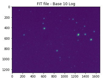
The same file but with a logarithm applied
However after taking the logarithm we were left with images with significant noise. The next step was to set a threshold intensity. Any value below this threshold would be changed to 0, and as a result we should be left with only stars and some hot pixels. We determined the optimum threshold value by taking the maximum of the second derivative of the total intensity.

Intensity values within a FITS file of M47

A graph of the 2nd derivative
For this image we found the optimum threshold intensity value to be 3.38.

The determined threshold applied to the log10 FITS file.
Since what we now had was just an array of points with different intensities, the next step was to cluster them into their own star arrays. First we used a Gaussian blur to smooth out the objects. This also had the additional benefit of blurring away the hot pixels.
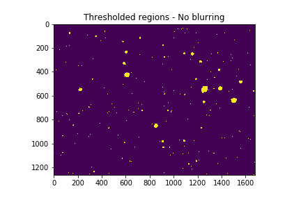
Here is a Boolean test demonstrating the thresholding applied to the image. Notice all the noise and jagged shape of the stars.
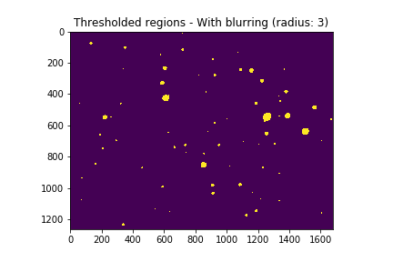
But with the Gaussian blur applied we have a cleaner image with much smoother objects.

Here we have an even larger blurring radius applied.
The next step was to cluster pixels into their own groups of stars. This was accomplished with the ndimage.label function.
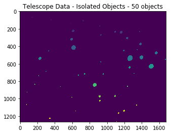
Here are the segregated objects. Each star has its own unique colour, indicating that it’s has it’s own distinct label.
Now that we had separated the intensities into their own stars, we could then work out the centre of masses for each one.
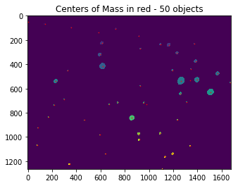
Centres of masses applied to the clusters
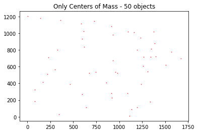
Centre of masses isolated
With the pre-processing complete, we could now work on automating the alignment of all the images with respect to each other.
