Written by Sara Fekri

Introduction

Hello everyone! We are the Telescope Group 2023: Sof, Stel, Sara, Sarthak, Elvi, Matin, and Malcom. As part of our 3^rd year research project, we are looking at different star clusters in London’s dark skies to measure the age of the stars within the clusters and produce a Hertzsprung-Russell (HR) diagram for them. 

Here, we will be presenting how the FITS files, an astronomy file format, are handled in Python and the steps taken to get the HR diagram of the star clusters. The objects we have captured are the open clusters Messier 35, Messier 36, and Messier 37 on the night of 08/February/2023. We also observed the Orion Nebulae M42, and globular cluster M3.

The steps taken for our project each have a detailed blog post and are as follows:

• The clusters observed 
• Handling FITS files 
• Removing hot pixels 
• Subtracting the background and stacking images
• Identifying stars and pairing them
• Computing the stars’ brightness and magnitude
• Plotting the HR diagram

HR Diagram

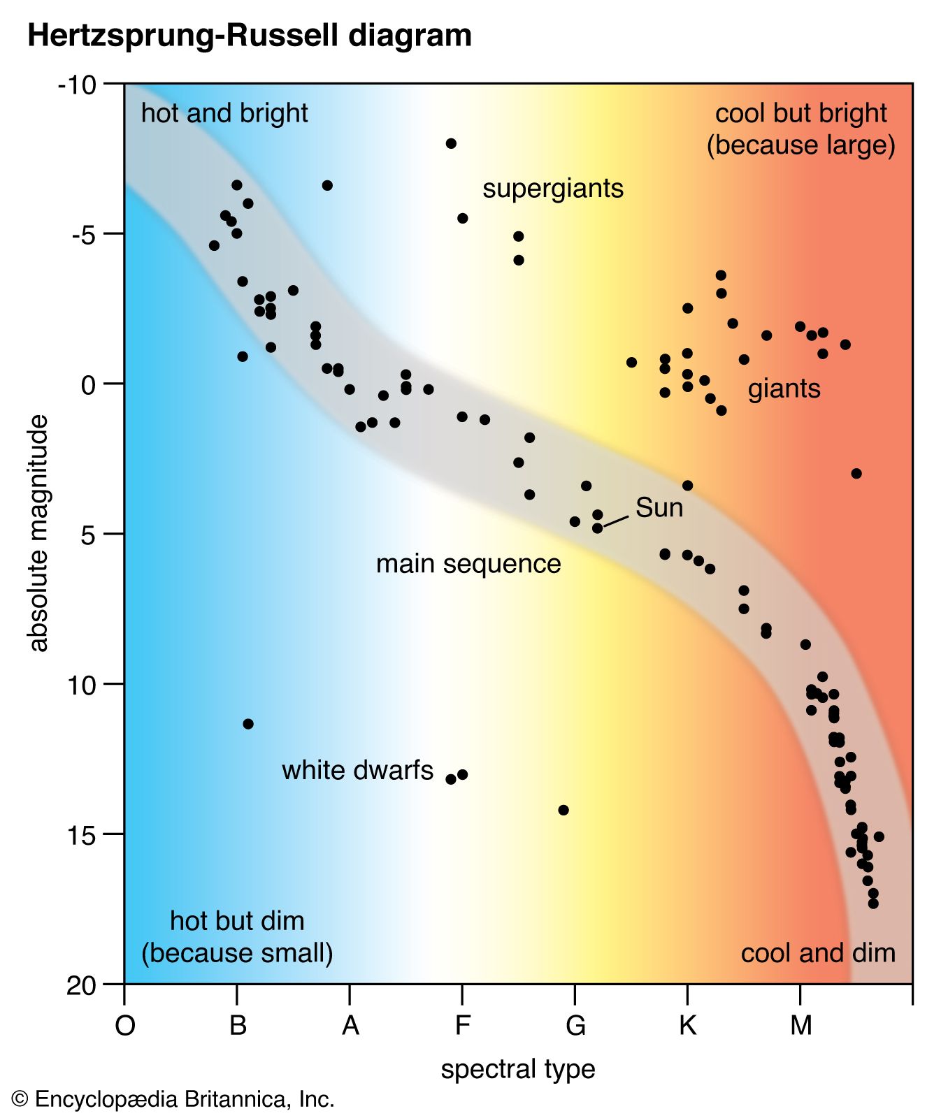
A Hertzsprung-Russell (HR) diagram is plot of stars showing the relationship between the stars’ absolute magnitude versus their effective temperatures. The absolute magnitude corresponds to the stars’ luminosities with negative values being brighter. The effective temperature can be shown using the stellar classification, where the stars from O to M correspond to decreasing temperate on the x-axis.¹

An important feature in the HR diagram is the main sequence (MS), the region where the primary hydrogen-burning takes place within a star’s lifetime. Looking into detail where the MS ends, the “MS turn-off”, gives astronomers information about the age of the star cluster.

The general layout of the HR diagram can be seen below, where stars of greater luminosity are located at the top of the diagram, and stars with higher surface temperature are towards the left side of the diagram. 

Our Cluster Data – M35

The data captured using the telescope at King’s gives us a FITS file, the most common digital file format in astronomy, and were captured with the blue and green filters attached. From that, we were able to open the files and get on with extracting the data. For this post, data from the M35 blue filter will be used. The raw image for M35_blue from Python can be seen:

However, this raw image does not only contain the stars; it includes hot pixels captured by the filters and a background. The histogram below shows the numbers of counts vs the pixels of the image above:

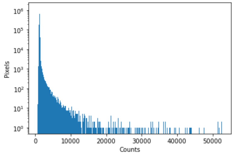
The brightest stars would be located on the histogram where the sharp peaks occur at the right of the curve. The highest peak of the histogram on the left side corresponds to the background of the image.

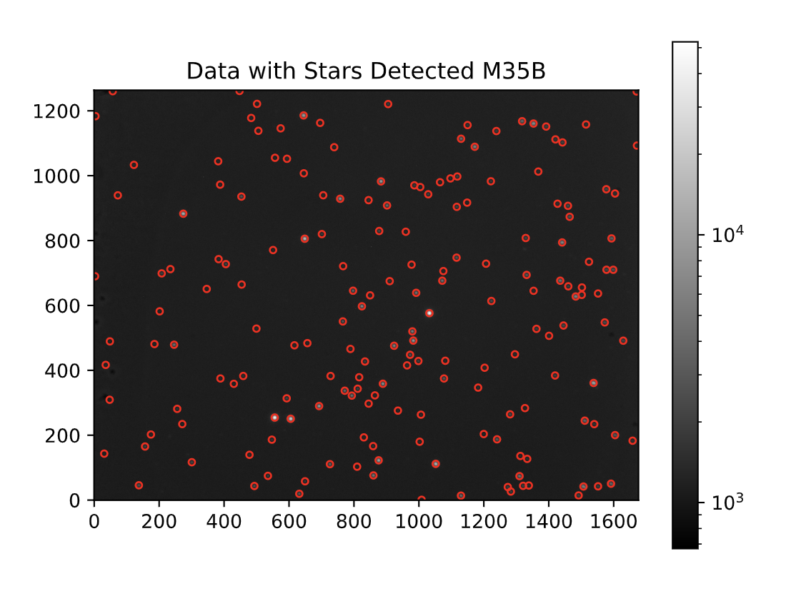
Next, the hot pixels needed to be removed from the image (detailed post here). Below is a picture showing the stars detected on the M35_Blue image after removing hot pixels using a code in Python:

The following procedure involved finding the background for it to be subtracted from each data set. The detailed methodology of background removal can be accessed here. The same steps were taken for each of the 10 data sets captured for M35_blue and M35_green. Now, the 10 images can be stacked to form:

The step afterwards was to identify the stars in the blue and green stacked images by comparing the two and see which stars overlap, i.e. correspond to the same star in the different filters.

After pairing the stars, the pixel counts of each star in both the blue and green images are found to compute the star’s apparent magnitudes (B and G). Finally, G vs. B-G is plotted, and this would form the observational HR-diagram of M35.

The plot above displays HR diagram of M35, where the Main Sequence branch is clearly shown. The MS turn-off point is where the stars leave the MS and form “Giants” which are seen on the top right of the diagram. Since most stars are on the MS branch, and there are very few giants, this concludes that the open cluster M35 is fairly young.

Conclusion

This project aimed to produce an HR diagram of M35 starting from extracting the data in the FITS files to comparing the stars in the stacked images of the blue and green filter. The same methodology was applied to M36 and M37. This post provided a summary of the steps taken to reach the final result where details can be found in the appropriate separate posts.

Hope you enjoyed reading!