
Written by Ceinwen Cheng
Betelgeuse, what used to be the 10th brightest star in the night sky, lies on the left shoulder of Orion’s constellation. This reddish star attribute’s its color to its classification of being a red supergiant around 15 times the mass of the Sun.
However, ever since October 2019, Betelgeuse’s apparent magnitude has had a drastic decrease that can be observed with the naked eye, dimming from an apparent magnitude of 0.6 in October 2019 to 1.8 in early February. The apparent magnitude scale is reverse logarithmic, i.e the lower the magnitude, the brighter the star. A star of apparent magnitude 1.0 is 2.512 times brighter than a star of apparent magnitude 2.0.

A graph published by Nature news article in February 26th c 2020 displaying a graphical representation of Betelgeuse’s apparent magnitude
Additionally, as recently as February 22nd, Betelgeuse has started brightening again, an increase of almost 10% from the dimmest point. There are many proposed explanations, one being a change in extinction and therefore not a change in the actual luminosity of the star, which is supported by the fact that the infrared observations have of Betelgeuse has barely changed since the dimming phenomenon. In astronomy, extinction is the absorption and scattering of light particles by cosmic dust between the observer and the light emitter.
We acknowledge several problems measuring the apparent magnitude of Betelgeuse in Central London, one of the most light polluted cities in Europe. If we measure Betelgeuse directly, our data will be skewed by a range of obscure interference such as clouds, atmospheric seeing, thermal turbulence, air and light pollution. These factors are hard to mitigate and could alter or change the trend of our data. Therefore, we approach this project by also tracking a star close to Betelgeuse that apparent magnitude isn’t changing much, Betelgeuse’s sister star Bellatrix. We are interested in the ratio of luminosity between Bellatrix and Betelgeuse.
Imaging both Bellatrix and Betelgeuse in 5 different sessions in 2020, on the 28th Jan, 3rd Feb, 11th Feb, 17th Feb, 2nd March 2020, we collected the images to be processed into a trend. Using Python 3, Dhruv Gandotra, our python expert, extracted the data from our images to produce the following trend in the graph below, showing the trend of the ratio of magnitudes between Betelgeuse and Bellatrix. Additionally, he also found a source online [twitter handle @Betelbot] that tracks the apparent magnitude of Betelgeuse over the same time frame as ours, allowing us to peer review our data.
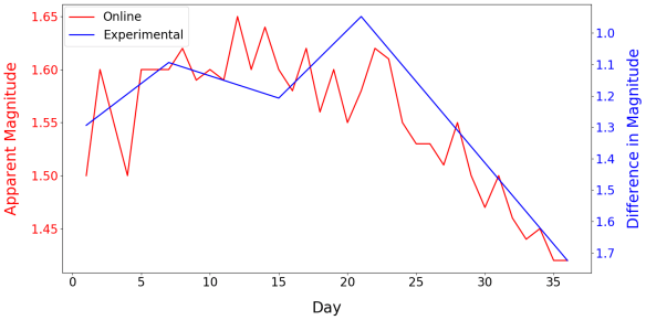
@Betelbot ‘s measure of Betelgeuse apparent magnitude (in red), compared to our experimentally calculated difference in apparent magnitude between Betelgeuse and Bellatrix inverted. Where Day 0 is the 28th Jan.
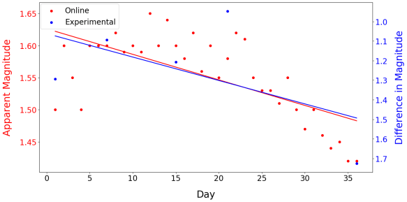
@Betelbot ‘s data and ours combined, with trend line calculated for both sets of data.
Brief Description of our code:
Importing our .fit files (a file format used in astronomy) into python, there are first and foremost several important points we need to take into account. All the images have noise, some images have hot pixels, and the position of the stars differ for each image. To solve these problems at the same time, Dhruv came up with an idea, to select a picture form a session, use an array to find the position of the maximum pixel brightness, then define a box around the star of fixed width, and only take data from that box. This way, any hot pixels can be cut out, the amount of noise will be relatively the same for the pictures in each session, and as the position of the stars do not move around too much, the star will still be in the box of data.
Note: We will be attaching parts of the code alongside its explanation for future references
After importing all our relevant modules into our code, we must first preview a single Betelgeuse image from the session, looking at the file’s information and then the data available in the file. From this we can extract the minimum, maximum, standard deviation, or mean of the pixel brightness.
Code:
#importing relevant modules
import numpy as np
import os
import math
from PIL import Image
import astropy
%config InlineBackend.rc = {}
import matplotlib
import matplotlib.pyplot as plt
%matplotlib inline
from astropy.io import fits

#opening single image and it's data
from astropy.nddata import Cutout2Dhdulist1a = fits.open(r"C:\Users\dhruv\Desktop\Project Pics\Betelgeuse\Session 1\betelgeuse_750.fit")
hdulist1a.info()
print(repr(hdulist1a[0].header))
data1a = ((hdulist1a[0].data)/256)

print('Min:', np.min(data1a))
print('Max:', np.max(data1a))
print('Mean:', np.mean(data1a))
print('Stdev:', np.std(data1a))
The next part of the code involves finding the position of the maximum pixel brightness i.e. where the star will be located, through an array. From this, we create a 50×50 cut out around the star, and graphed the cut out. Now that we have a preview on an image, we can repeat this easily for the 10-15 other images taken per session, add all their data and find the mean average of their data.
Code:
#locating position of star and creating a cut out
position1 = (223, 248)
size1 = (50,50)
cutout1a = Cutout2D(np.flipud(data1a), position1, size1)
plt.imshow(np.flipud(data1a), origin='lower', cmap='gray') #using np.flipud as the image is inverted
cutout1a.plot_on_original(color='white') #displacing the position of the cut out in the image
plt.colorbar()

#plotting cut out
plt.imshow(cutout1a.data, origin='lower', cmap='gray')
plt.colorbar()

#importing the rest of the images taken in the session
hdulist2a = fits.open(r"C:\Users\dhruv\Desktop\Project Pics\Betelgeuse\Session 1\betelgeuse_751.fit")
hdulist3a = fits.open(r"C:\Users\dhruv\Desktop\Project Pics\Betelgeuse\Session 1\betelgeuse_752.fit")
hdulist4a = fits.open(r"C:\Users\dhruv\Desktop\Project Pics\Betelgeuse\Session 1\betelgeuse_753.fit")
hdulist5a = fits.open(r"C:\Users\dhruv\Desktop\Project Pics\Betelgeuse\Session 1\betelgeuse_754.fit")
hdulist6a = fits.open(r"C:\Users\dhruv\Desktop\Project Pics\Betelgeuse\Session 1\betelgeuse_755.fit")
hdulist7a = fits.open(r"C:\Users\dhruv\Desktop\Project Pics\Betelgeuse\Session 1\betelgeuse_756.fit")
hdulist8a = fits.open(r"C:\Users\dhruv\Desktop\Project Pics\Betelgeuse\Session 1\betelgeuse_757.fit")
hdulist9a = fits.open(r"C:\Users\dhruv\Desktop\Project Pics\Betelgeuse\Session 1\betelgeuse_758.fit")
hdulist10a = fits.open(r"C:\Users\dhruv\Desktop\Project Pics\Betelgeuse\Session 1\betelgeuse_759.fit")
hdulist11a = fits.open(r"C:\Users\dhruv\Desktop\Project Pics\Betelgeuse\Session 1\betelgeuse_760.fit")
hdulist12a = fits.open(r"C:\Users\dhruv\Desktop\Project Pics\Betelgeuse\Session 1\betelgeuse_761.fit")
hdulist13a = fits.open(r"C:\Users\dhruv\Desktop\Project Pics\Betelgeuse\Session 1\betelgeuse_762.fit")
hdulist14a = fits.open(r"C:\Users\dhruv\Desktop\Project Pics\Betelgeuse\Session 1\betelgeuse_763.fit")

#extracting the data of each image
data2a = (hdulist2a[0].data)/256
data3a = (hdulist3a[0].data)/256
data4a = (hdulist4a[0].data)/256
data5a = (hdulist5a[0].data)/256
data6a = (hdulist6a[0].data)/256
data7a = (hdulist7a[0].data)/256
data8a = (hdulist8a[0].data)/256
data9a = (hdulist9a[0].data)/256
data10a = (hdulist10a[0].data)/256
data11a = (hdulist11a[0].data)/256
data12a = (hdulist12a[0].data)/256
data13a = (hdulist13a[0].data)/256
data14a = (hdulist14a[0].data)/256

#stacking the images and plotting
sum1 = data1a+data2a+data3a+data4a+data5a+data6a+data7a+data8a+data9a+data10a+data11a+data12a+data13a+data14a
average1 = sum1/14
ax1a = plt.plot(average1)
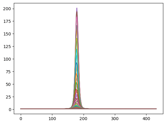
All 14 of the images of Betelgeuse taken in session 1 stacked, where the x axis is the number of pixels???, and the y-axis is the relative mean average brightness of?? the stacked images.

The graph above shows the cut out relative to the actual image taken of Betelgeuse in Session 1.

This graph displays the actual cut out, where we shall be focusing on taking our data from.
An interesting thing we can find in our stacked image is the amount of background noise there is, which can be seen if we reduce the y-axis stacked data to a limit of 1.10 to 1.50. Background noise is light registered by the CCD from a space in the sky where there are no light sources. Background noise is often caused by light diffusion or scattering in our atmosphere, and telescopes in space such as the Hubble Space Telescope do not encounter such a problem.
Code:
#changing the y-axis of the graph to show noise
ax1a = plt.plot(average1)
plt.ylim(1.1,1.5)

A zoomed in graph of the earlier stacked images to a y-axis limit of 1.10 to 1.50, displaying the noise present in the images.

This is the sum of the stacked cut out data after converting the image into an array. One thing to point out is that there are to be two peaks, i.e. the position of the star moved. This does not change anything as we are finding the summed maximum pixel brightness.
Code:
#repeating finding the position of the star and creating cut out for the stacked image
position2 = (224, 253)
size2 = (50,50)
cutoutf1 = Cutout2D(np.flipud(average1), position2, size2)
plt.imshow(np.flipud(average1), origin='lower', cmap='gray')
cutoutf1.plot_on_original(color='white')
plt.colorbar()
plt.imshow(cutoutf1.data, origin='lower', cmap='gray')
plt.colorbar()
xf1 = cutoutf1.data
ax1b = plt.plot(xf1)
mn1 = np.sum(xf1)
print(mn1)

print('Min:', np.min(xf1))
print('Max:', np.max(xf1))
print('Mean:', np.mean(xf1))
print('Stdev:', np.std(xf1))
Finally, we convert the stacked images into an array, and sum all the data, as seen in the graph above. The curve we produced is seen to be a nice Gaussian distribution. As we are looking for the ratio of apparent brightness between Bellatrix and Betelgeuse, we do not need the apparent magnitude. The whole process is repeated for Bellatrix, and then the sum of the respective data is placed into a ratio and normalised 2.512 (due to the reverse logarithmic scale of apparent magnitudes), to give the experimental difference in apparent magnitudes.
Code:
#where mn1 is the sum of brightness for Betelgeuse and mn2 for Belletrix
mn1/mn2
#finding the difference in apparent magnitude
a = math.log(mn1/mn2,2.512)
print a
((a-1.22)/1.22)*100  #percentage error
Graphs of Interest

Discarded stacked data graph of failed session, with a hot pixel seen as a green line on the left.

The same graph with the y-axis reduced to 1.0-3.5 mean photons received in 0.1 s seconds. Still observing the hot pixel as well as an increase in noise past the x-axis 535 pixels mark.
When using the telescope, the CCD (Charged-Coupled device) needs to be cooled, up to around -31ºC. However, the graphs above shows the result of taking images when the CCD is not sufficiently cooled, in this image, the camera was cooled to around -7ºC. Hot pixels occur when the camera sensor heats up, an electrical charge is leaked, resulting in a pixel that is much brighter than expected. In our data, there is an obvious hot pixel, as there is a pixel that is very bright but not located at where the star is, additionally, there is no Gaussian spread in it neighbouring pixels. The hot pixel should go away after the CCD is sufficiently cooled.
Rapidly cooling the CCD may cause ice crystals to form in the detector, often dry ceramic pills placed in the detector to reduce the amount of moisture. On the far right of our data graphs, we see one of the stacked photos have a large amount of noise compared to the other photos. A few plausible explanations for such a phenomenon: ice crystals forming due to the CCD rapidly cooling, or a naughty undergrad using their phone near the telescope, increasing the background luminosity.
Summary
The span of our allocated project time is minuscule compare to many astronomical events. The dimming of Betelgeuse occurred over 4-5 months and should still be monitored in the future due to it sudden brightening. By the time this blog is published, we have only taken 5 session of images of Betelgeuse and Bellatrix, and to produce a trend or a timeline worth looking at, we need many more sessions and images. Clouds remain our worst enemy. Springtime in London brings rain and cloudy days, and we cannot image on a cloudy night.
However, even though Malcolm dislikes the company of optimists, there are still a few more weeks before the end of the allocated project time, where we will continue imaging Betelgeuse and Bellatrix in hopes of providing you with a more complete trend of Betelgeuse’s dimming and brightening.
